Mathematical Explanation
Variational Autoencoder

This article was created for those who would like to understand more about the mathematical reasoning behind a model such as VAE. For this purpose I am introducing a range of different concepts in statistics that help understand the decision-making of this paper's authors. I sum- marized only the most relevant mathematical statements for this post of each topic. To make a VAE more comprehensive I emphasized on the modeling of it and core concepts to computationally realize it. Aditionally, I used day-to-day examples and visualisations that help building an intuition. If you have any questions or suggestions regarding this topic feel free to contact me.

Required knowledge

The following topics are necessary to understand this article:

Analysis 1,2 & 3
Probability theory 1
Basic statistics
Basic Deep Learning

I will recap some necessary core concepts from the following topics:

Bayesian Belief Network
Bayesian inference
Variational inference
Monte Carlo Estimate

If you are keen to know more details about each topic I can suggest:

_config.yml

Introduction

This article elaborates on relevant concepts and approaches mentioned in the paper Auto-Encoding Variational Bayes by Diederik P. Kingma, Max Welling.

To understand the architecture of a VAE, a generator, and its mathematical model, we will need to determine first the goal of such a model type and its relationship to a discriminator.
With a discriminative model we want to make a prediction about an attribute based on various observations. Such a model tries to learn a mapping from that data to this attribute. To do so it tries to extract features of these observations that has the highest correlation with that attribute.

Imagine, when I was a little child, I always got upset when my mom bought apples that had some brown spots. She always answered: “No, they are good! Those are just some injuries.” Sure, as if apples are like humans and could have “injuries” - you are just trying to make these cheap apples palatable, was my response back then. Indeed, my mom was right, injuries of the apples skin exposes its tissue to oxygen that turns polyphenol (a micronutrient in the apple) into melanin.

Coming back to our problem, we could collect observations, like skin color of an apple and its surface structure and so on, to make a prediction whether an apple is rotten or not. And, even though my mom was right, brown spots are usually a good indication since some infecting spores of fungi that occur in rotten apples create a brown coloration. A discriminator would be able to find that correlation, like me as a child.

Unfortunately, such a model will eliminate also apples that are healthy to consume but are just a bit damaged. Because of those instances, a model that can learn the causal relationship is of course more precise. To achieve that it would have to learn the generating process of decaying apples. [1]

The goal after training is that such a generator creates **realistic data**, here a realistic example of an apple, therefore it needs to be able to understand what realistic means.

If we abstract this case, we could say that an attribute like the level of decay is just another feature that describes an object. From that perspective every object is a state of a collection of features or call it attributes if you like.

Based on my observations and assumptions I did as a child I would have described such an apple by the following states of features:

mainly red colored
brown spots
shiny skin
decomposed
etc.

A trained generator for this application should 'understand' that the occurrence of having a shiny skin and being decomposed at the same time is highly unlikely. In other words, a generator should /c/uncover how all the features that describe an object are jointly distributed/c/.

The idea of generating realistic data can be expanded:

Let’s say we have a trained generator at hand that understands the generating process of building sentences. That means it understands that there is first an idea that is afterwards expressed in a sentence. But an idea exists within a context. So how would we incorporate such a context? An intuitive approach would be to say: Given we speak about rotten fruits and I asked “Is this apple healthy to consume?” what would be a realistic response? Such a contextual information is thereby incorporated by conditioning the input data on it.

Another important goal of training a generator is data completion. For instance, image resolution. For this purpose we need to transform the generator also into a conditional generator. It generates data depending on the state of some additional data, here a low-resolution image. [4]

Often in ML we encounter the problem of having just a very small dataset that is labelled. A generator can also help in those instances. For this purpose you let a deterministic model train parallel to the generator. The labels are then treated like features, such that the discriminative model has to predict the labels as features but also other useful descriptive features. Based on these predicted labels and features the generator has to reconstruct the original data. [5]

In summary, such a model should be used for **semi-supervised learning**, **data completion** and **generating realistic data**. And it does so by learning the joint distribution of all features.

_config.yml

REMARK

Every illustration was designed by me and every mathematical statement was (re)formulated and every calculation was done by me. Obviously these statements and calculations are backed up by the sources I have mentioned in the last chapter and my mathematical background.

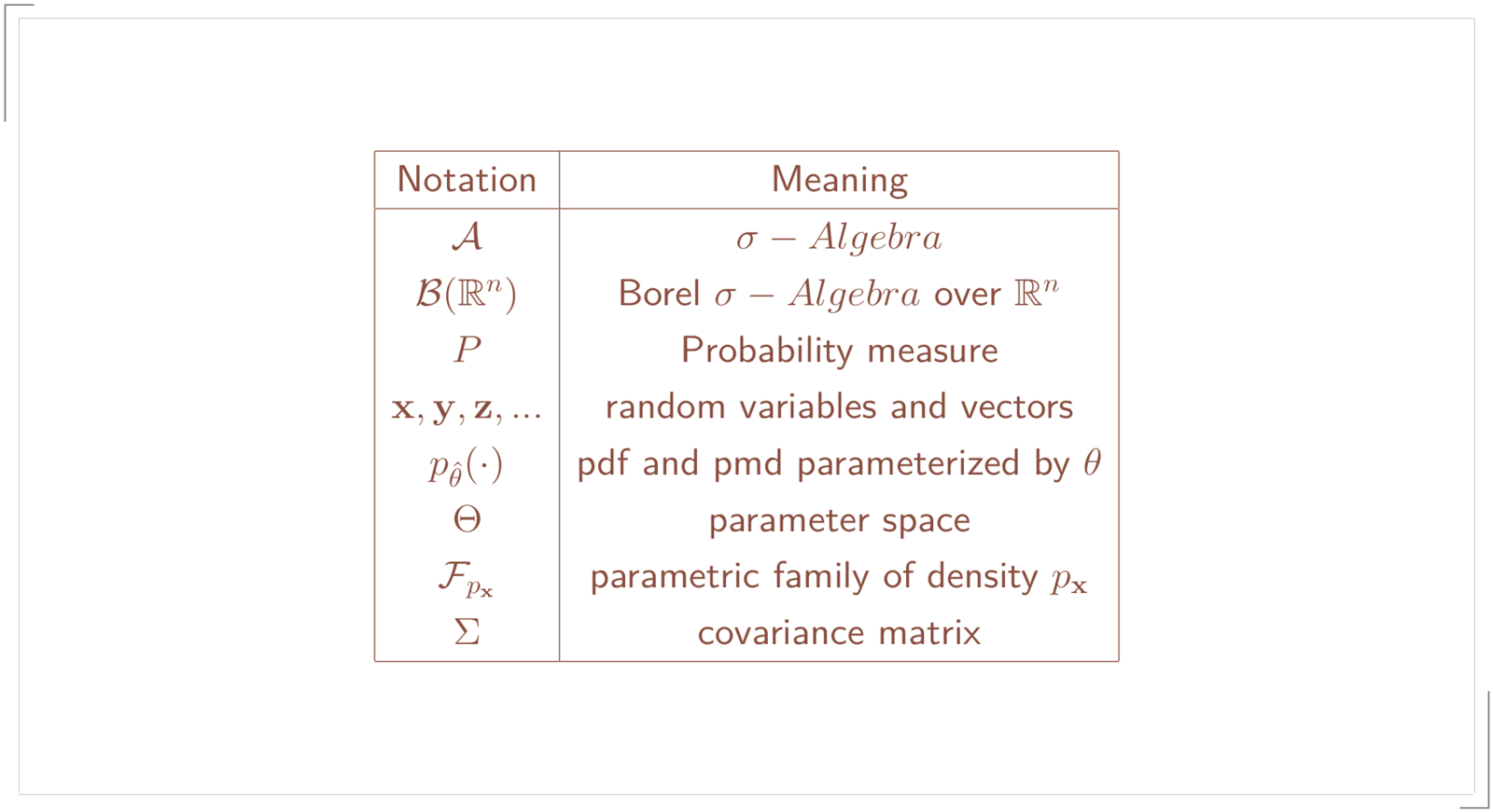
NOTATION

I usually use capital letters to denote random variables or vectors and f to denote probability density functions compared to p for probability mass functions. Since the authors of the VAE paper chose to use small letters for random variables and vectors and p for both probability density and mass function I decided to stick with that notation.

_config.yml

Modeling

Some of you may know that /c/finding a good data representation/c/, that is extracting more expressive features of the data, will increase the chances of training a good discriminator. Typical methods include the use of an auto-encoder or principal component analysis which finds a representation of the data where each feature is uncorrelated. A new representation of a datapoint is called **latent feature vector**. The word, latent, stems from the fact that the space of latent features in a DL model for data representation is hidden from us.

_config.yml

On the left you can see a generators output for creating handwritten numbers. By varying the feature values we will obtain different results as you can see on the left image.

Let’s first formulate that mathematically:

_config.yml

Next, we want to build a /c/neural network that parametrizes this joint distribution/c/. To achieve this I want to introduce the concept of a Bayesian Belief Network: A **Bayesian Belief Network** is a directed acyclic graph where each node is a random variable and the edges (arcs) are the densities. It is useful to display the conditional relationships between each random variables.

_config.yml

Bayesian inference

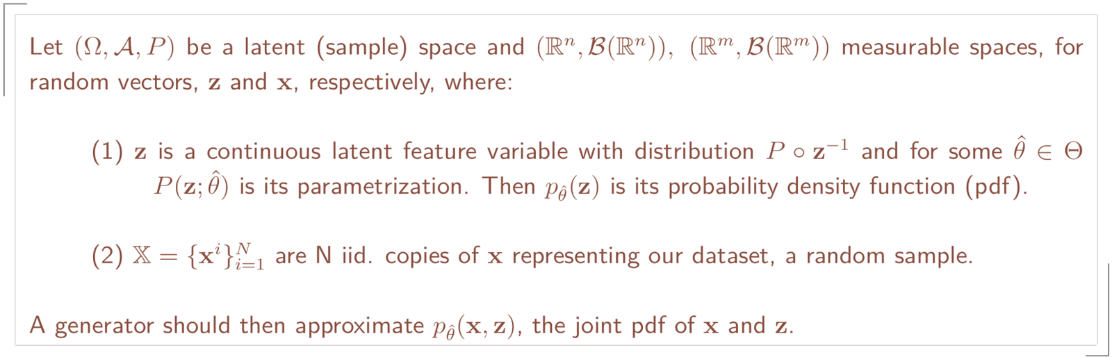
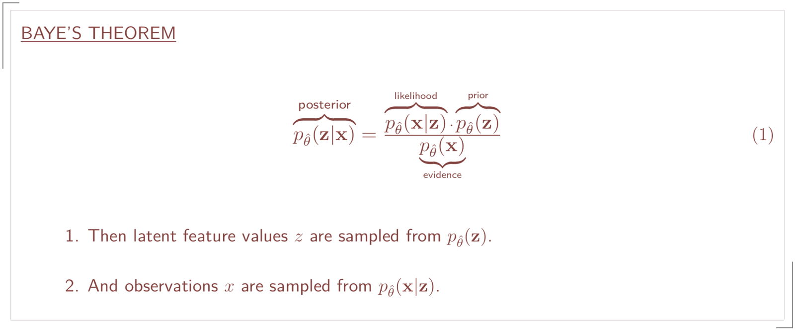
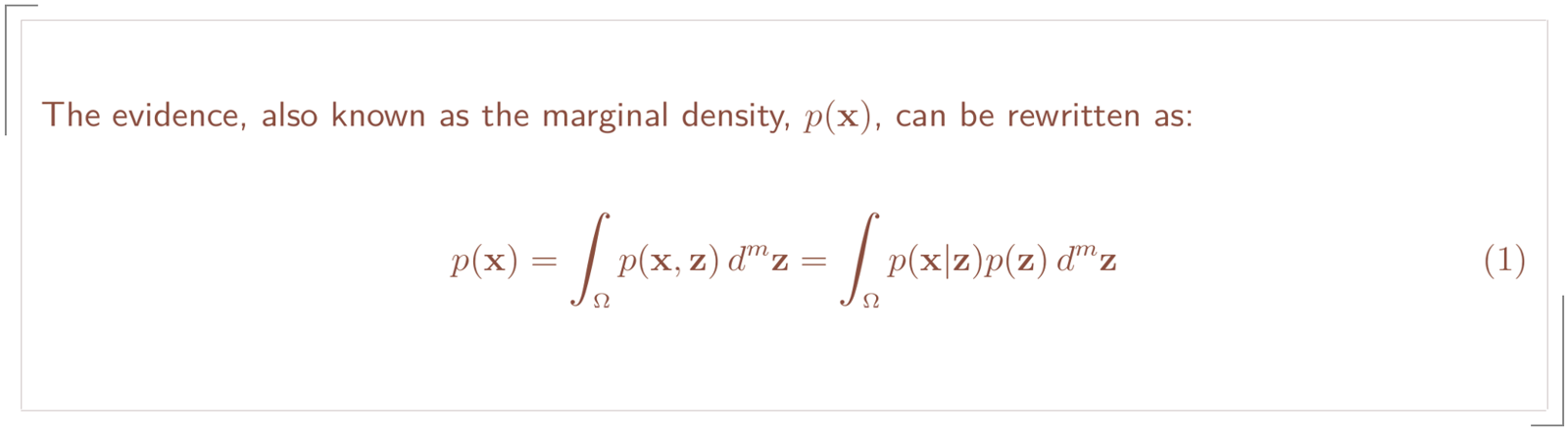
Since we do not know the pdf of the latent vector but might have some **prior knowledge** or we made an initial assumption about its distribution we can use Bayesian inference to /c/update prior distribution by the posterior/c/.

_config.yml

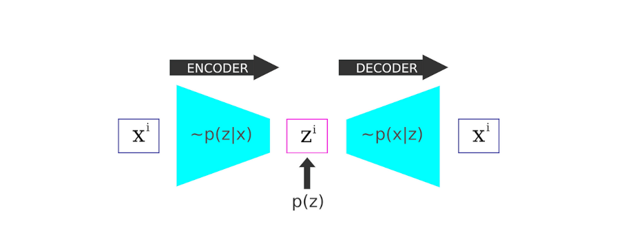
The product of the likelihood and prior is our model. At this point we are just missing the evidence, p(x). We can obtain it by marginalizing it from the joint distribution as we will later see. This update principle will set up the architecture and mechanism of a VAE.

_config.yml

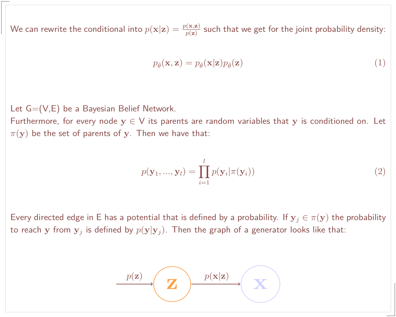
The VAE architecture

To obtain the **likelihood** a neural network learns its distribution during training while we need to assign another neural network with the task to learn the distribution of the **posterior**. The latter type of neural network is called an inference model. For this purpose, the Variational Auto-Encoder uses /c/an encoder to parametrize the posterior and a decoder to parametrize the likelihood/c/.

The following illustration captures this mechanism:

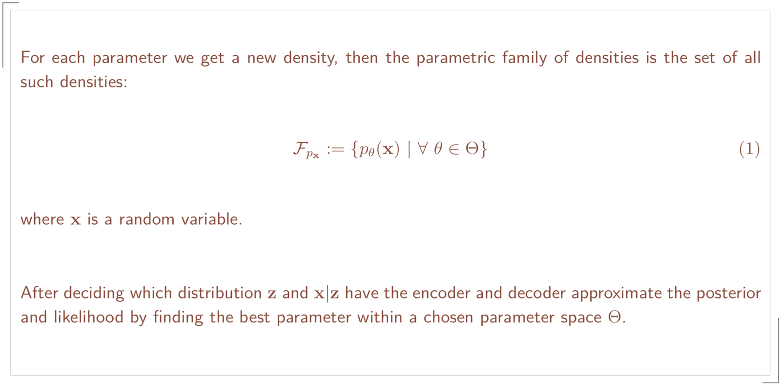
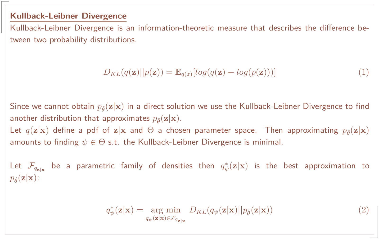
This diagram illustrates assignments of distributions.

To understand the learning process for this model I will need to introduce you to the concept of a family of densities:

_config.yml

For unsupervised and semi-supervised learning the authors of this paper suggest to assume a **multivariate Gaussian**. Since a multivariate normal distribution has a **mean vector** and for this model suggested **diagonal covariance matrix** as its parameters the /c/inference model, here an encoder, has to define them to describe the posterior/c/. I will later on go further into detail.

An explanatory illustration that shows the model design.

_config.yml

Intractability

For Bayesian inference we have seen already that calculating the posterior requires the knowledge of **the evidence**. Unfortunately, it is usually intractable:

_config.yml

Either this integral has no closed-form solution due to the complexity of the data or the likelihood function is too complex due to nonlinear hidden layers. That means /c/we need to find a loss function that does not require the knowledge of the evidence/c/.

_config.yml

Variational inference

**variational inference** will bring us closer to the solution. It is /c/a method that approximates the posterior distribution through optimization/c/. The basic approach is to create a family of possible densities and with a distance measure to find the density from this family that is the closest to the one we want to approximate.

[2]

_config.yml

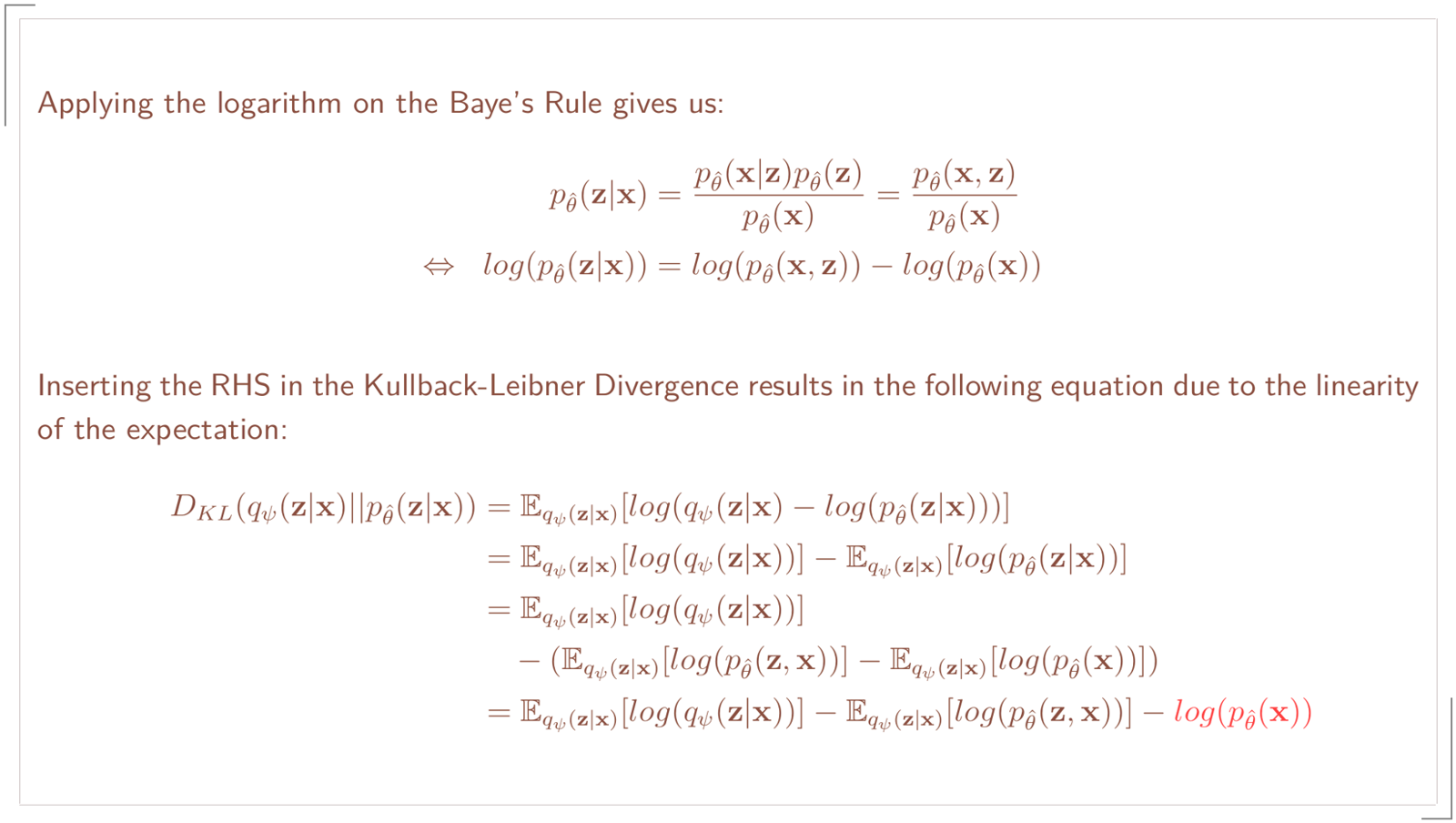
Equation (2) is by itself not computable in our case because it involves calculating log(p(x)). The following calculation will show that:

_config.yml

As we can see, /c/that optimization problem contains the log of the evidence which makes it not computable/c/.

_config.yml

The Evidence Lower Bound

Even though the Kullback-Leibner Divergence is not computable we can use it after applying some tweaks.

_config.yml

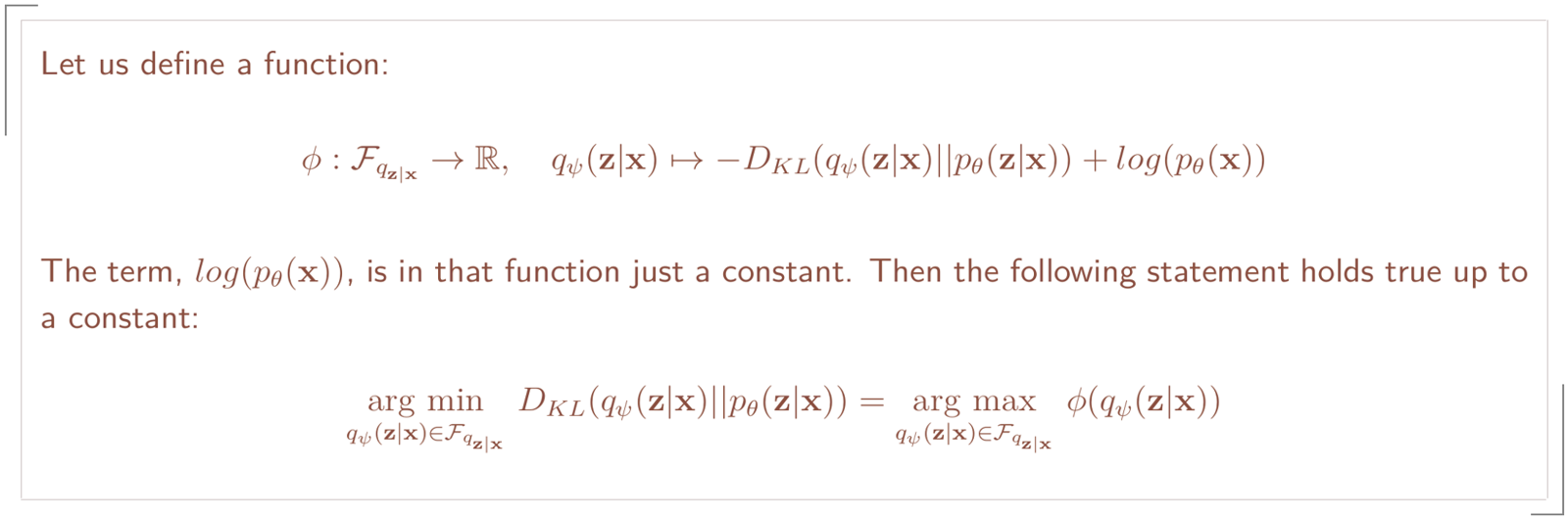
By adding the log(p(x)) term to the Kullback-Leibner Divergence we eliminate log(p(x)) from our objective. With some further transformations we obtain an objective that we can use for our model.

_config.yml

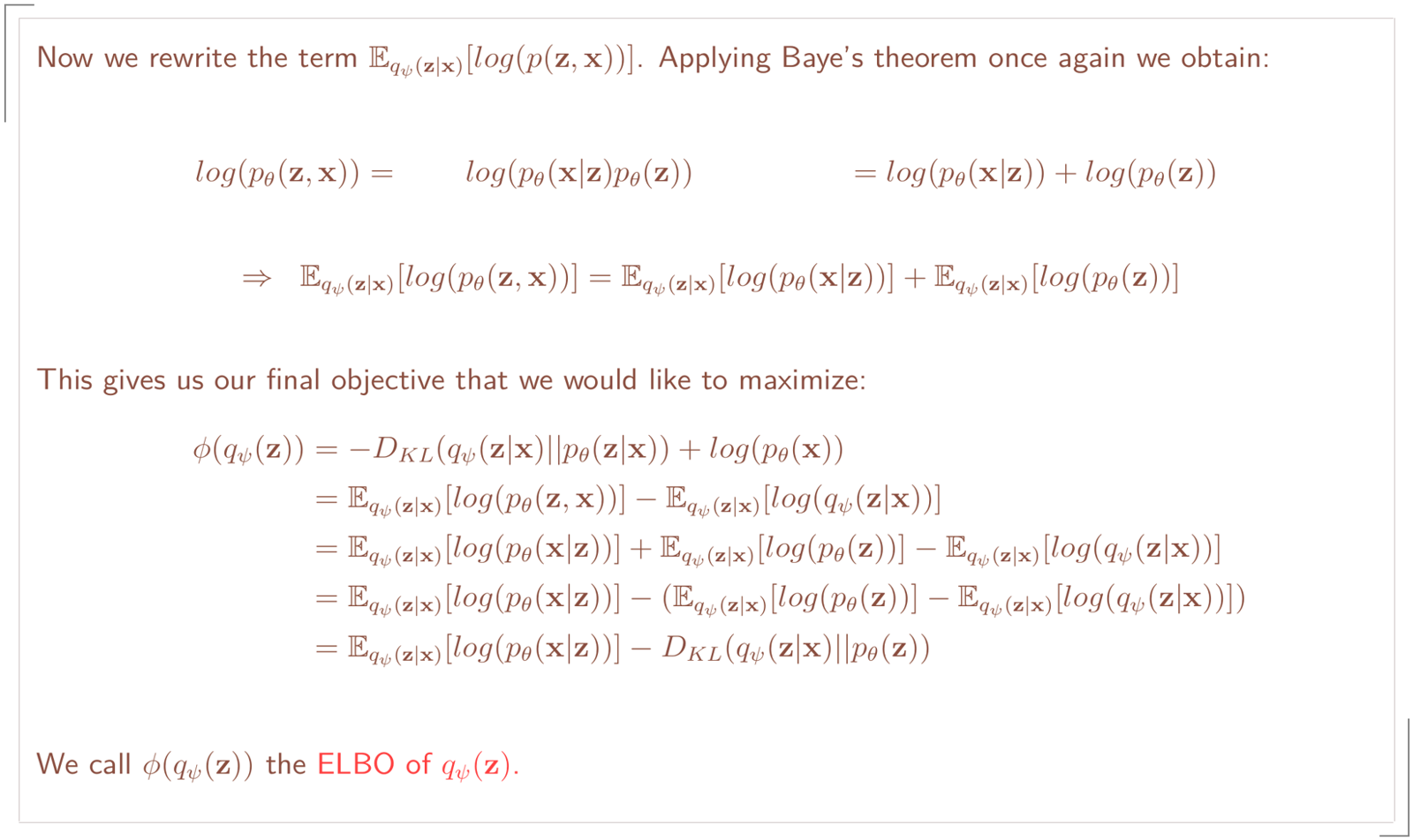
With that new expression we only have to work with the prior, likelihood and posterior. From the following property we can see the reason why it is called the evidence lower bound.

_config.yml

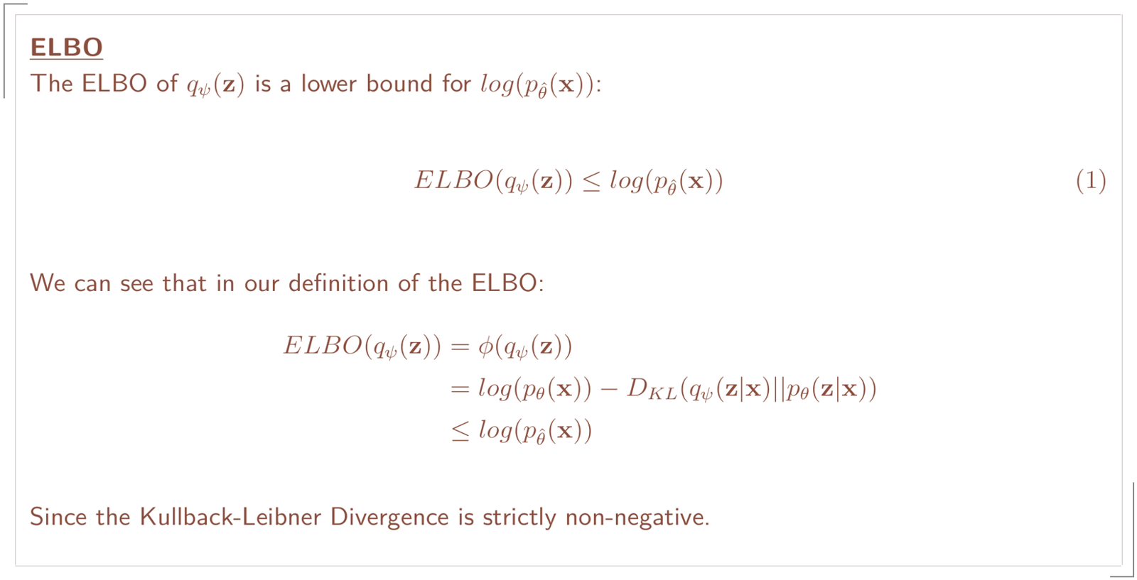
Below you can find an animated example where p is a normal density function and q a gamma density function. The gamma distribution is very flexible and, hence, useful to derive many different distributions like the chi-square, exponential and beta. The plot on top is the graph of the ELBO and below a plot of p and q with varying values for its parameters. The maximum of log(p) is zero for every density and since the ELBO is bounded from above by log(p) the ELBO is therefore bounded by zero from above.

_config.yml

The ELBO is also viewed as the **reconstruction error** minus the Kullback-Leibner Divergence.

/c/To get the maximizer of the ELBO via stochastic gradient decent we need to differentiate it w.r.t. the variational parameters φ and generative parameters θ./c/ That can be a bit tricky as we will see in the next chapters.

_config.yml

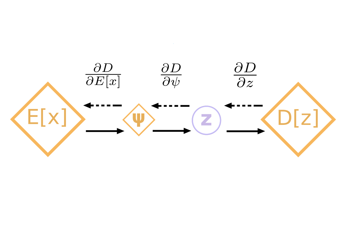
The gradient problem

After constructing our loss function we need to find a method to train our model. Kingma and Welling intend to use stochastic gradient decent, which is a noisy estimation of the true gradient. This method requires calculating the gradient which leads us to two problems:

I) This model needs to sample latent values from z, a random vector, and feed it to the decoder. During **backpropagation** the model will encounter the issue that /c/z cannot be deterministically expressed/c/ and thereby cannot calculate the gradient. There are two main approaches, Black-Box Variational Inference (BBVI) and the Reparameterization Trick, to overcome this learning obstacle.

II) Whereas the Kullback-Leibner Divergence is analytically tractable - the reconstruction error is most often not. This creates of course an issue when the model needs to calculate the gradient of it. A typical solution would be to use **Monte Carlo estimates**.

/c/The gradient estimates of BBVI typically suffer from high variance/c/ and that would require using a very small learning rate which lead to slow convergence. Therefore, the second approach is recommended. This method typically needs only one Monte Carlo sample to estimate a noisy gradient.

_config.yml

Reparameterization Trick

The idea is to find a /c/deterministic expression of the random vector, z/c/. This is achieved by constructing a **differentiable bijection** between z and a random noise, ε, that does not depend on the variational parameters.

_config.yml

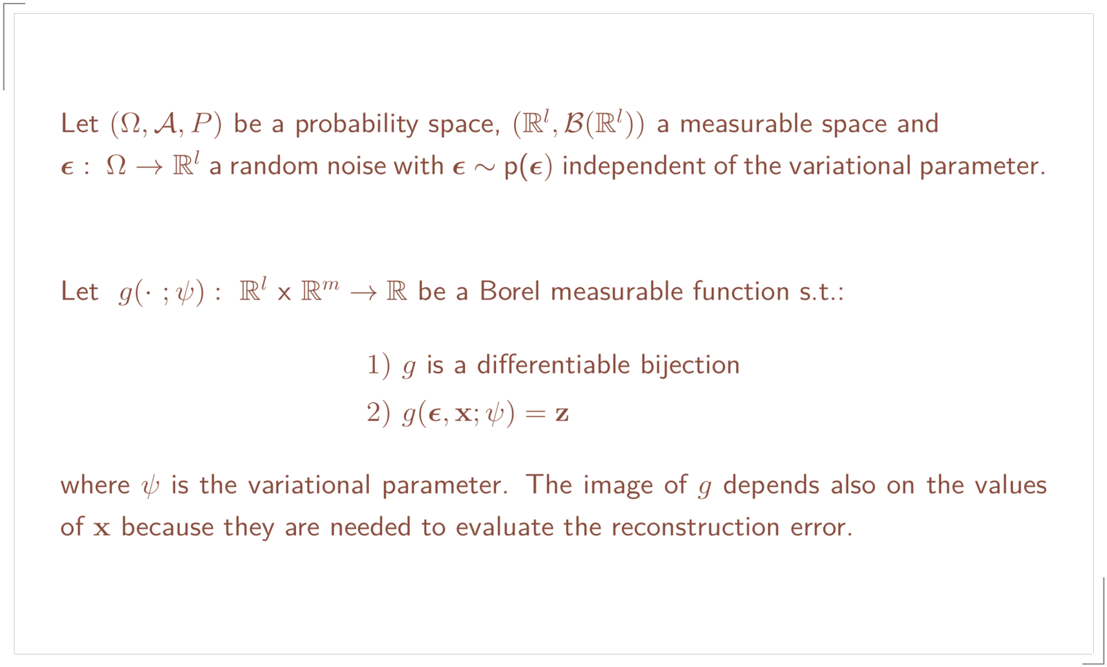
As you might have noticed g depends not only on the random noise, ε, but also on x. That is because we sample z from q(z|x). Then the Reparameterization Trick will give us the following identity:

_config.yml

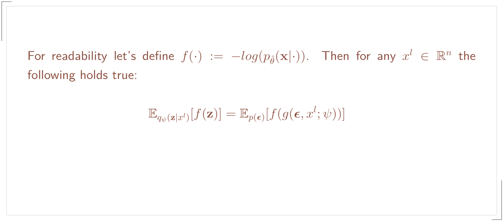
For those who know this identity can now jump the next proof. We didn’t learn that identity in probability theory 1. So here it goes: The concept of this proof is based on the transformation theorem for the expectation.

_config.yml

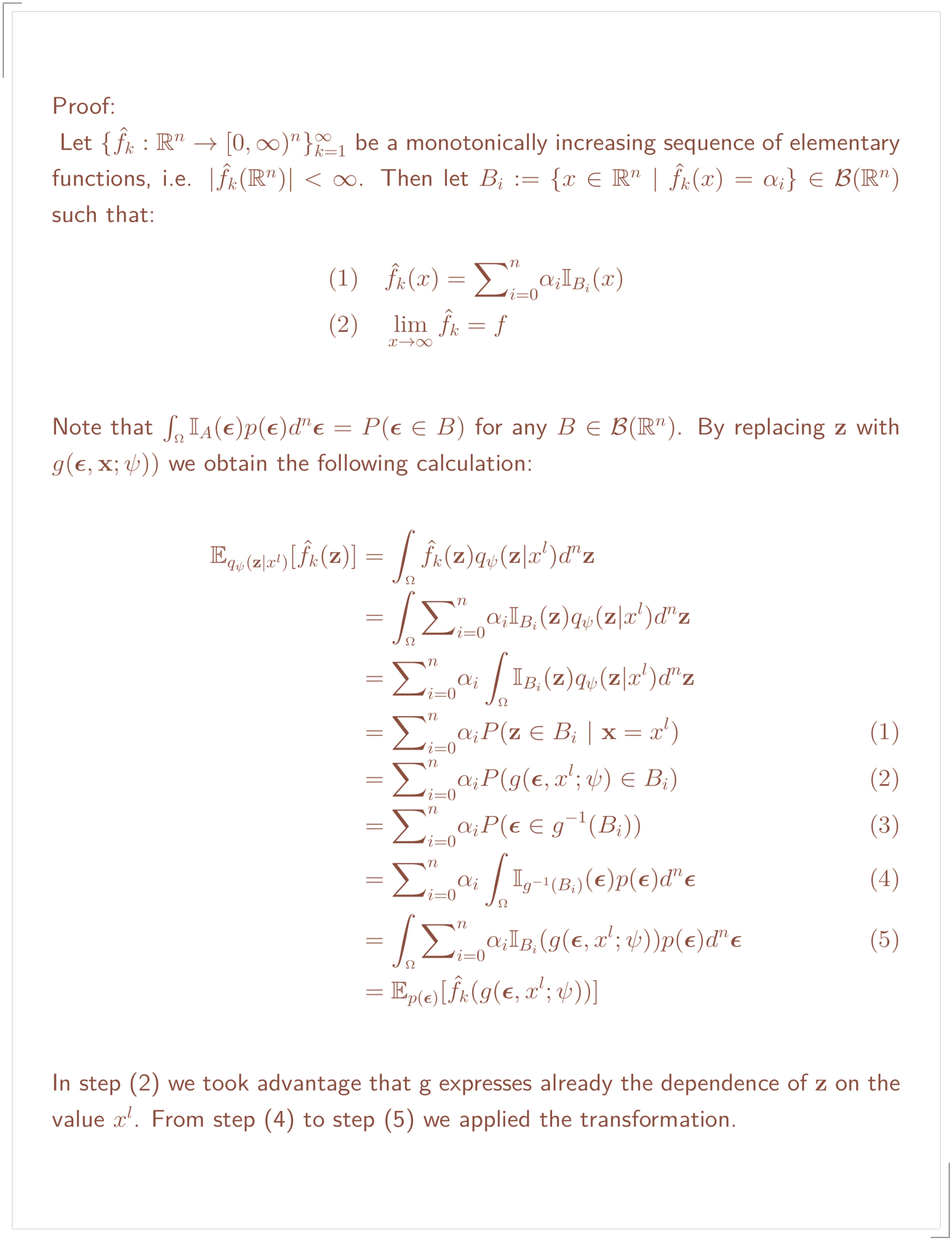
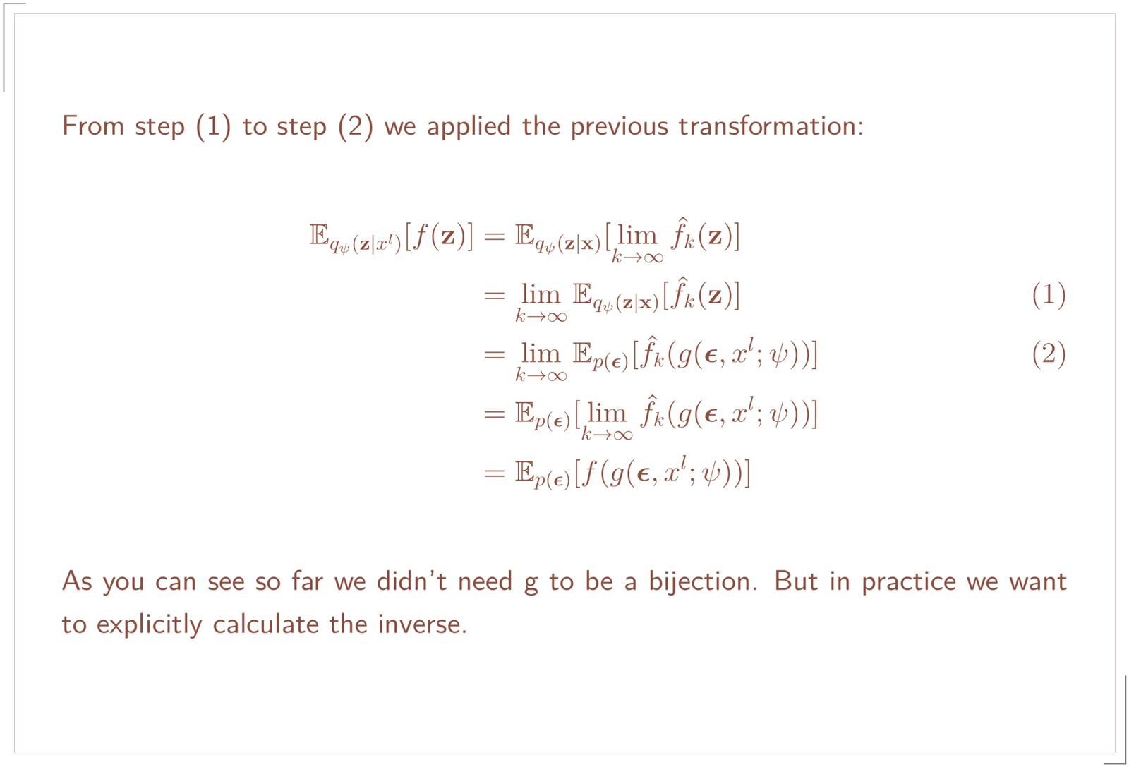
From Beppo Levi’s theorem we know for our sequence of functions we can take the integral before the limit and then by taking the limit over these sequence of elementary functions and again applying Beppo Levi we will get our identity:

_config.yml

Due to the linearity of the expectation we simply multiply it by -1 to obtain -f(z) = log(p(x|z)).

_config.yml

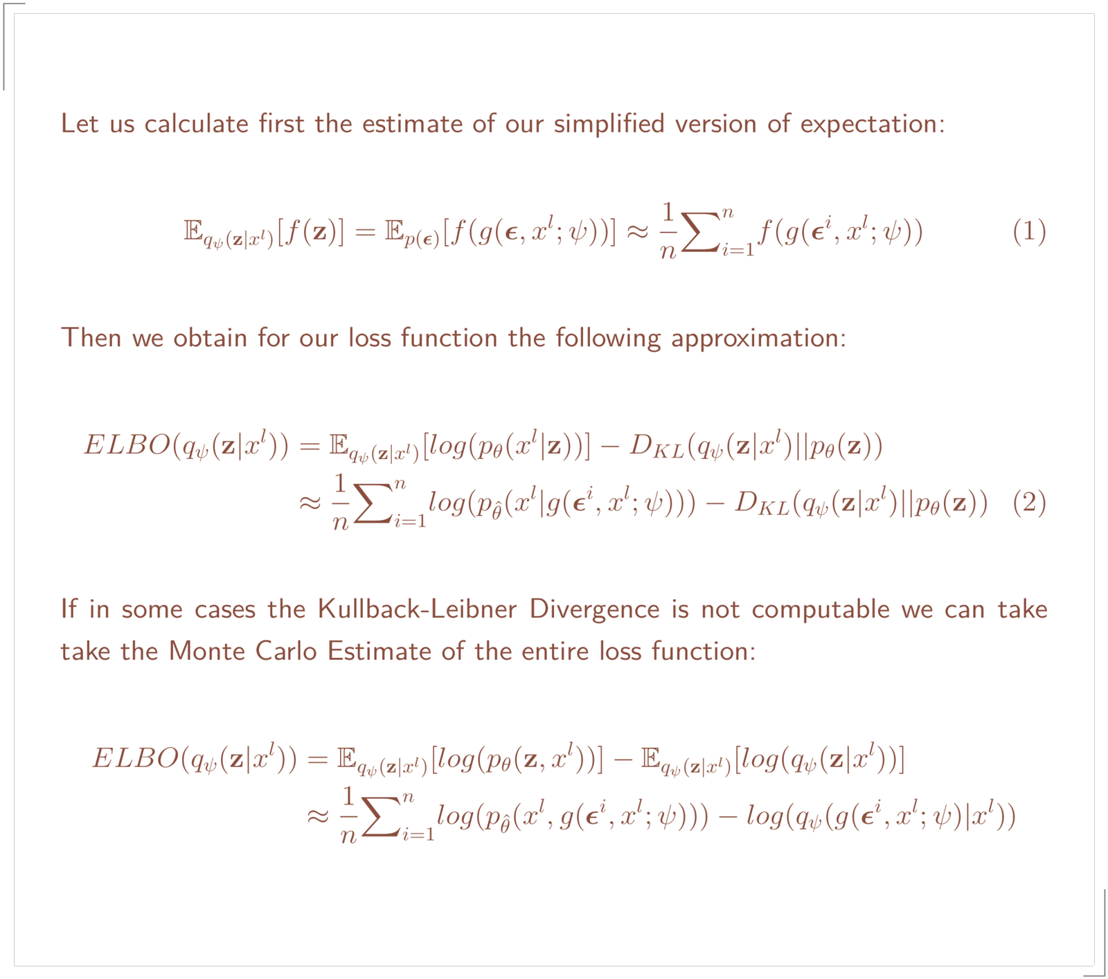
Monte Carlo Estimator

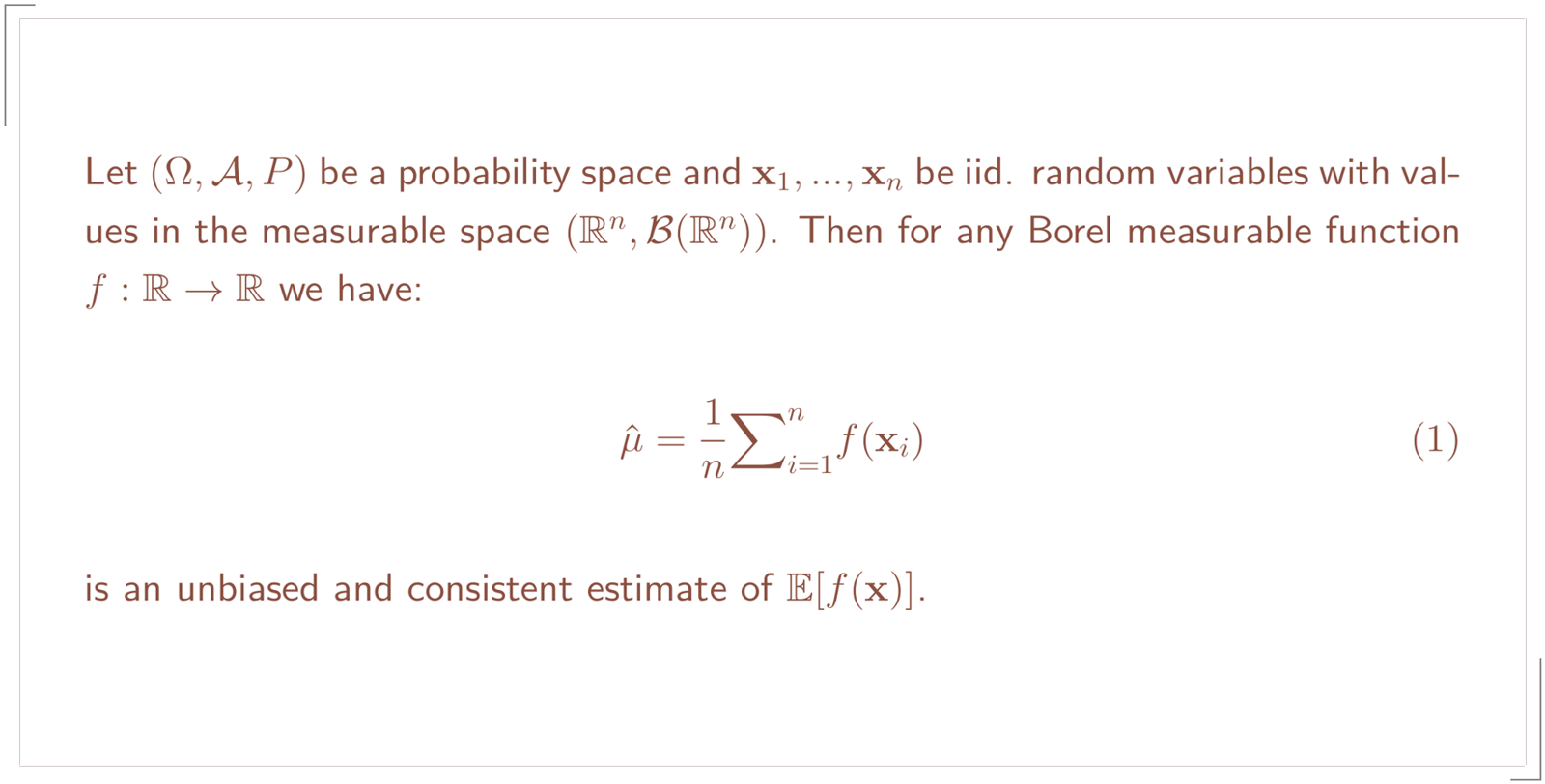
The basic /c/Monte Carlo Estimate approximates the transformed expectation/c/. We are interested in such approximations when this **expectation is intractable** to compute exactly as it is in our case. There are also other approximations like Markov Chain EM but this method requires repeated sampling and for large datasets this becomes very quickly inefficient.

_config.yml

We want to use this estimate of our reparameterized expectation:

_config.yml

However, /c/reparameterization is not as generic as BBVI/c/. It is typically used with Gaussian variational distributions and does not easily generalize to other common distributions, such as the **Gamma or Beta**, without using further approximations.

[3]

_config.yml

G-REP

Francisco J. R. Ruiz and David M. Blei developed the **generalized reparameterization** (G-REP) gradient.

The requirements to apply G-REP are:

sampling from q(z|x) can be done efficiently
q(z|x) is differentiable w.r.t. z and Ψ.

Applying their generalized version yields a transformation that makes p(ε) independent of Ψ in at least its first moment.

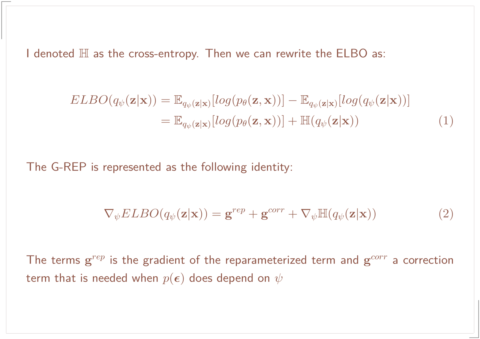
Their /c/gradient estimator is a combination of the reparameterization-trick that we have calculated before and the gradient estimator of the BBVI/c/:

_config.yml

In the next section I will show you the BBVI gradient and the reparameterized gradient in comparison. Afterward I will show you how the G-REP contains both terms. For simplicity, I reduce the case to the unconditional distribution.

_config.yml

Coming back to the G-REP method it is represented by the following terms:

_config.yml

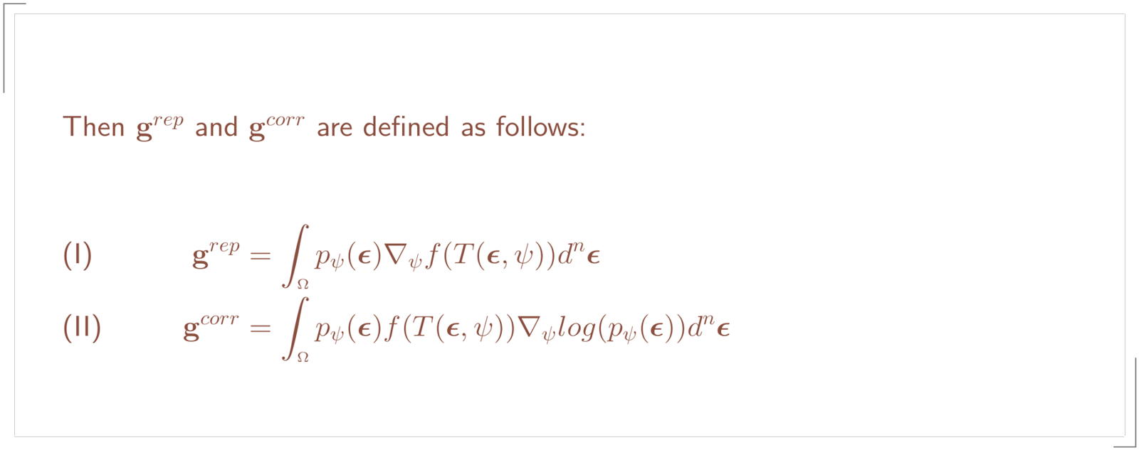
The $g^{rep}$ term is nothing else then the reparameterized expectation just writen out as an integral. By some restructuring of our objective we can derive them as a sum:

_config.yml

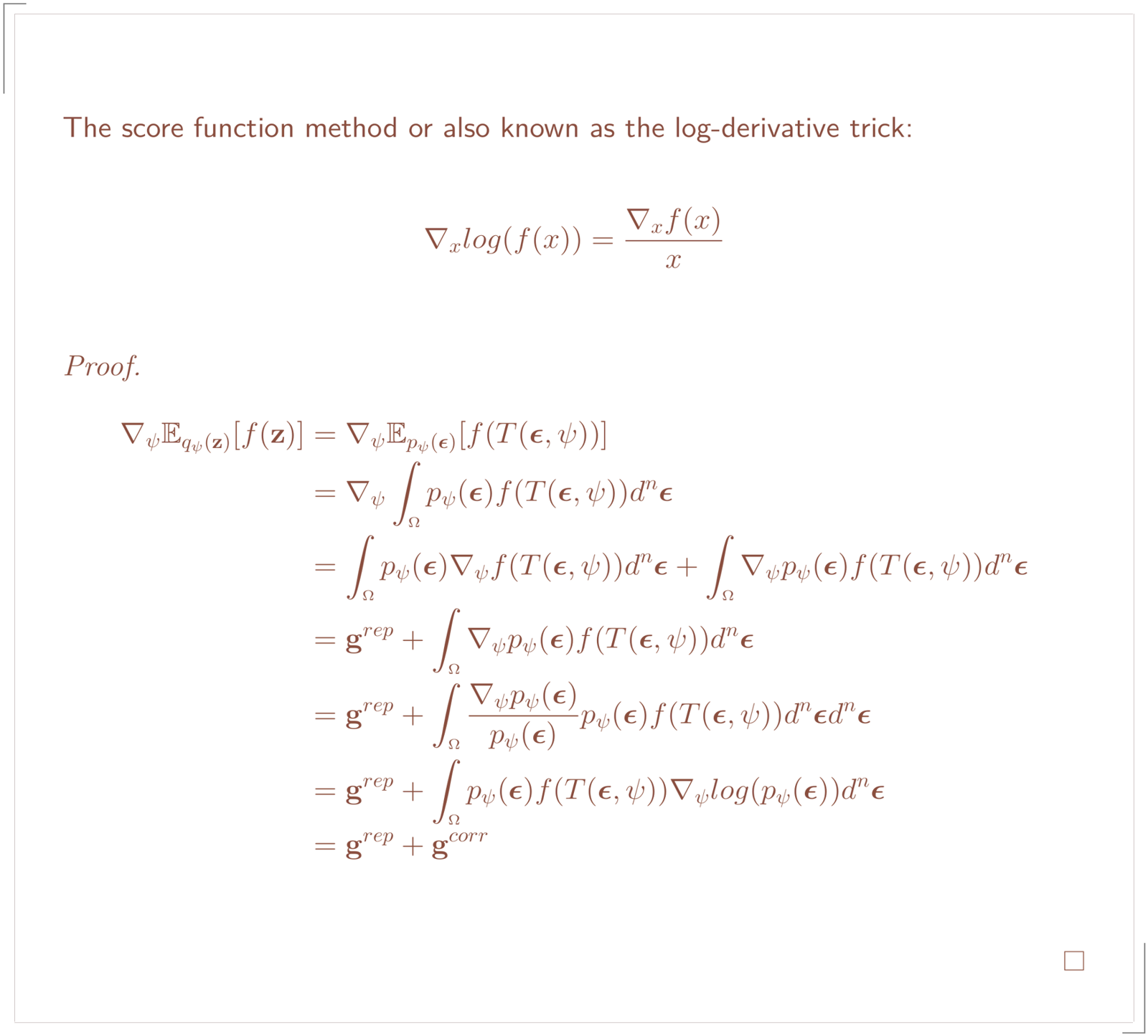
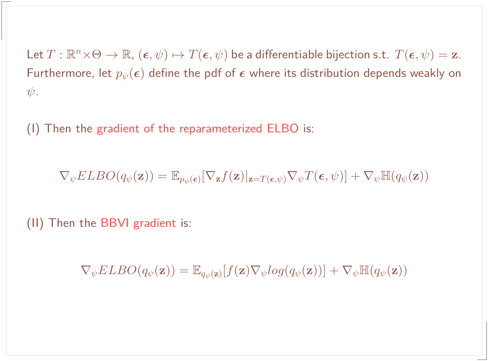
In the next section I show you how you can retrieve the BBVI gradient as well as the gradient of the reparameterized expectation:

_config.yml

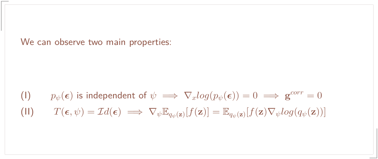
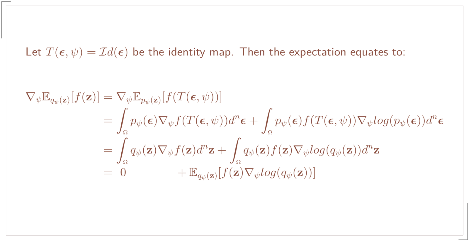
Due to the first property we can obtain the gradient of the reparameterized expectation. The latter property shows that we can retrieve the BBVI gradient when we choose T to be the identity.

_config.yml